Example of an SQ file for Sysquake

Programs for Sysquake, called SQ files, implement only the definition of figures and how the user can interact with them. Sysquake provides itself support for synchronizing the figures, zoom, undo/redo, and file management.

To show you how simple they can be, here is an SQ file which displays in the same figure the magnitude of the frequency response of a continuous-time system, and the same system sampled at a frequency you can manipulate with the mouse. The Shannon theorem, which states that the sample frequency should be at least two times higher than the bandwidth of the signal to be sampled in order to avoid loosing information (i.e. there should be enough samples to catch the fastest changes), and the aliasing which occurs when it is not verified, are much easier to understand than with a mathematical demonstration or with static figures.

Here is the code of this SQ file:

variable Ts      // sample time

init Ts = init   // init handler for initial values

figure "Frequency Response"       // new figure definition
draw drawFreq(Ts)                 // draw handler
mousedrag Ts = dragFreq(_id, _x1) // manipulation handler

functions
{@
function Ts = init
  Ts = 0.2;
  subplots('Frequency Response');

function drawFreq(Ts)
  scale('linlin/logdb', [0,20*pi]);  // default scale
  Ac = poly([-2,-1+10j,-1-10j]); // continuous-time t.f.
  Bc = Ac(end);                  //  defined by its poles
  bodemag(Bc, Ac);               // plot freq. response
  (Bd, Ad) = c2dm(Bc, Ac, Ts, 'z');  // -> discrete time
  dbodemag(Bd, Ad, Ts, 'r');     // plot freq. response in red
  line([1,0], pi / Ts, 'b', 1);  // plot Nyquist freq. in blue
                                 //  which can be manipulated

function Ts = dragFreq(id, x)
  if ~same(id, 1)                // not the Nyquist frequency
    cancel;                      // cancel the drag
  end
  Ts = pi / x;                   // new sample time
@}

Open this file in Sysquake, move the Nyquist frequency (half the sample frequency, displayed as a vertical blue line) with the mouse, and here is what you will observe:

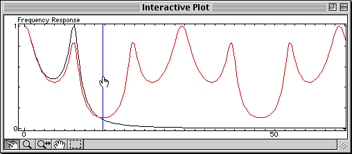
The lower the Nyquist frequency, the worse the sampled signal (in red) approximates the continuous-time signal (in black).