sampling.sq

Effect of sampling a signal with different conversion methods

Automatic control and signal processing is usually performed using digital computers, microcontrollers or programmable logic. This offers much more flexibility than analog devices. For good results, sampling must respect the Shannon theorem, which states that sampling should be performed at at least twice the frequency of the bandwidth of the sampled signal; otherwise, aliasing (high-frequency signal components appearing at lower frequencies) occurs. When a digital computer is connected to a system, the output is usually sampled by picking the measured values at regular discrete times, and the input is usually applied at the same times and kept constant until the next sample time; this operation is called a zero-order hold.

Another operation consists in converting a continuous-time transfer function (describing the frequency filtering of a system between its input and its output) to a discrete-time transfer function. When the transfer function corresponds to a filter or a controller, the zero-order hold method is usually not used, because there is no such hold; the problem is different, and actually it has no exact solution. Usually, the s operator of the Laplace transform is approximated with finite differences, or the poles and zeros of the Laplace transform are mapped to the complex plane of the z transform.

First contact

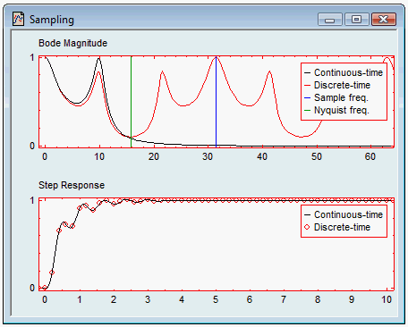
When you open sampling.sq from Sysquake (menu File/Open), two figures are displayed: the frequency response magnitude and the step response. Each figure shows a third-order continuous-time system in black, and its discrete-time equivalent in red. The discrete-time transfer function is obtained with a zero-order hold, which gives an exact match for the step response. In the frequency response figure, the blue line represents the sampling frequency, and the green line the Nyquist frequency. You can move them to the right or to the left to change the sampling frequency. Observe the samples which stay on the continuous-time step response, and the aliasing effect when the sampling frequency is too small. Aliasing is related to the sparse samples, which cannot reproduce the oscillations.

Figures

Bode Magnitude

The magnitude of the continuous-time transfer function is displayed in black, and the magnitude of the discrete-time transfer function is displayed in red. The Nyquist frequency and the sampling frequency, which can be manipulated, are displayed as green and blue vertical lines, respectively.

Bode Phase

The phase of the continuous-time transfer function is displayed in black, and the phase of the discrete-time transfer function is displayed in red. The Nyquist frequency and the sampling frequency, which can be manipulated, are displayed as green and blue vertical lines, respectively.

Step Response

The step response of the continuous-time transfer function is displayed in black, and the samples of the step response of the discrete-time transfer function are displayed as red circles. The samples can be dragged to the right or to the left to change the sampling period.

Continuous-Time Poles

The poles of the continuous-time transfer function are displayed as crosses in the complex plane of the Laplace transform. The stability region (to the left of the imaginary axis) is shown in yellow.

Discrete-Time Poles

The poles of the discrete-time transfer function are displayed as crosses in the complex plane of the z transform. The image of the stability region in the complex plane of the Laplace transform is shown in yellow; it depends on the method used for the conversion to discrete time.

Settings

Zero-Order Hold

The discrete-time transfer function is obtained by adding a zero-order hold element before the transfer function and sampling the result.

Tustin

The discrete-time transfer function is obtained by performing the following substitution in the continuous-time transfer function:

s = 2/Ts (z-1)/(z+1)

where Ts is the sampling period.

Back Rect

The discrete-time transfer function is obtained by performing the following substitution in the continuous-time transfer function:

s = 1/Ts (z-1)/z

For Rect

The discrete-time transfer function is obtained by performing the following substitution in the continuous-time transfer function:

s = 1/Ts (z-1)

Pole/Zero Matching

The discrete-time transfer function is obtained by replacing the poles and zeros p of the continuous-time transfer function with exp(p Ts). If necessary, zeros are added at the origin to reduce the delay to one sampling period.

Continuous-Time TF

The continuous-time transfer function can be entered in a dialog box as two vectors containing the coefficients of the numerator and denominator, respectively, highest power first.

Sampling Period

A precise value can be entered in a dialog box for the sampling period.