Sysquake Pro – Table of Contents

Sysquake – Table of Contents

Sysquake for LaTeX – Table of Contents

GPC.sq

Design of a linear Generalized Predictive Controller

A GPC (Generalized Predictive Controller) is a controller which minimizes the error between the desired future set-point and the predicted system output. The predicted output is based on a model of the system, the past input (control signal) and output (measures), and the future control signal. Minimizing the future error leads to the "best" sequence of future control signal samples. Only the first sample is actually used; other ones are discarded, and a new optimization is performed for the next sample, to take into account as well as possible the past disturbances though their effect on the measured output. With the GPC, the system input is supposed to be constant after some time, called the control horizon Nu. The optimization is performed over a finite prediction horizon, from t+N1 to t+N2. The cost function J to be minimized is

where u(t) is the control signal, y(t+k|t) the prediction for output at time t+k made at time t, r(t+k) the future set-point, supposed to be known in advance, and lambda a non-negative fixed parameter whose purpose is to reduce the amplitude of the changes of control signal and make the minimum always unique. In GPC.sq, lambda is set to a small fixed value.

First contact

When you open GPC.sq from Sysquake (menu File/Open), two figures are displayed: the open-loop step response and the closed-loop step response. The system is non-minimum-phase, second-order, stable, discrete-time, and has a delay of 15 samples. In the open-loop step response, the control horizon is displayed in red, and the prediction horizons in red. They can be changed by being dragged with the mouse. The closed-loop step response is displayed with the set-point; both are delayed, so that the non-causal output is null before t = 0. Observe the very good tracking when you increase the control horizon by dragging the red line to the right and you enclose the first oscillation of the open-loop step response between the prediction horizons by dragging the right blue line to the right. Observe also the bad transient effect when you increase the lower prediction horizon to exclude the first oscillation. If the prediction horizon is too small, the controlled system may become unstable.

Figures

Open-Loop Step Response

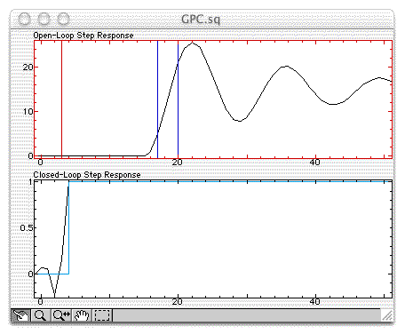
The open-loop step response of the system is displayed in black. The control horizon is displayed as a red vertical line, and the prediction horizon as two blue vertical lines. For best results, the range delimited by the prediction horizon should include at least the first oscillation of the system step response. The horizons can be manipulated.

Closed-Loop Step Response

The closed-loop step response of the controlled system is displayed in black, and the set-point (step) is displayed in light blue.

Closed-Loop Input Response

The input (control signal) of the closed-loop step response of the controlled system is displayed in black.

Closed-Loop Poles

The closed-loop poles are displayed as crosses in the complex plane, and the closed-loop zeros are displayed as circles. Note that for high-order systems, such as those with large delays, the numeric computation of roots may give inaccurate or totally wrong results.

Settings

System

The transfer function of the system can be given in a dialog box as two polynomials, highest power first. Systems with delays have poles at 0, i.e. trailing zeros in the list of denominator coefficients.

Input Weight

The input weight lambda (non-negative scalar) can be set in a dialog box.