Disponible uniquement en anglais

Sysquake Pro – Table of Contents

Sysquake – Table of Contents

Sysquake for LaTeX – Table of Contents

MPT.sq

Modern Portfolio Theory

To choose a portfolio, i.e. to decide how much one should invest in each of the possible assets, one typically considers not only their rate of return, but also their risk. This results in a multi-objective optimization problem with a set of Pareto-optimal solutions (i.e. solutions where an objective criterion cannot be improved without losing on another criterion). SQ file MPT.sq displays this set, also known as the Markowitz efficient frontier.

First contact

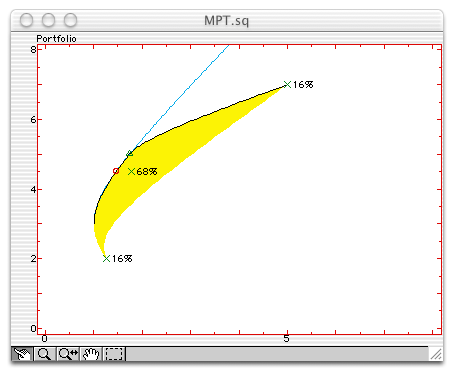
The set of assets is characterized by the mean of each asset and their covariance matrix. The figure represents the assets, the efficient frontier and the portfolio in a plane where the vertical axis is the rate of return and the horizontal axis is the risk as a standard deviation (both in percents). Each asset is displayed as a cross; the efficient frontier is the black line; and the portfolio is the red circle. You can drag the portfolio on the efficient frontier. The percentage of each asset is displayed near the corresponding cross. Some information is displayed in the status region when you point an element with the mouse. The yellow region represents the set of portfolios which can be obtained. By default, you can only buy assets up to 100 %; if you remove this constraint by unselecting "Positive Assets Weights" in the Settings menu, the feasible region is larger and permits better portfolios (more return and less risk), but you may have to sell what you do not own to have the cash required to buy a larger amount of another asset. The light blue line represents this larger region.

With the initial values, assets are not correlated, and you can move them freely in the rate-of-return/risk plane.

Figures

Portfolio

The only figure displays all the available information. The feasible region is displayed in yellow; its upper left border, always convex, is the efficient frontier and is displayed in black. Assets are displayed as red crosses and can be moved with the mouse if they are not correlated (i.e. if the covariance matrix is diagonal). The portfolio is displayed as a red circle and can be moved on the efficient frontier. If only positive asset weights are allowed, the frontier of the feasible region without this constraint is displayed in light blue; corner portfolios (portfolios on the efficient frontier where an asset is positive on one side and null on the other side) are displayed as green triangles. When the mouse is over an asset, in addition to its rate of return and its risk, its beta is displayed. The beta of an asset is defined as

  beta = cov(asset, portfolio) / var(portfolio)

Settings

Investments

A dialog box is displayed, where you can specify the rate of return of the assets (an n-by-1 vector) and their covariance matrix (an n-by-n symmetric matrix).

Positive Asset Weights

If set, the weight of all assets is constrained to be nonnegative, which reduces the size of the feasible region.

Corner Portfolio Display

If set, the corner portfolios are displayed with green triangles (see above for their definition).

Market Line Display

The market line is a straight line tangent to the efficient frontier and starting from the risk-free asset. It is the efficient frontier of the set of assets including the risk-free asset. The tangent point is the market itself, i.e. a portfolio which can be combined with the risk-free asset and generate any point of the market line.

Considering the risk-free asset separately has the advantage of permitting another interpretation. Let r0 be the risk-free rate-of-return. The tangent point is the portfolio which minimizes the probability to have a rate-of-return smaller than r0 (Roy criterion).

The market line can be manipulated either by dragging the portfolio (red circle) or the risk-free asset (blue square).

Risk-free Rate of Return

A dialog box is displayed, where you can enter the rate of return of the risk-free asset.

Weight Display

When selected, the weight of each asset is displayed as a percentage.

Whole Feasible Region Display

When selected, the whole feasible region is calculated and displayed in yellow. Otherwise, only the left part is displayed (in black for the efficient frontier and in yellow for the lower part). Note that there is a right limit only if asset weights are constrained to positive values. Calculating the right frontier is not very useful, because what we are interested in is minimizing the risk. However, it provides a more accurate picture of the problem.

References

MPT.sq is based on "La théorie moderne du portefeuille", by Florin Aftalion, Patrice Poncet, and Roland Portait, PUF, Ed. "Que sais-je?", Paris, 1998.